Bayesian Learning Explained
Bayes theorem, prior, likelihood, posterior — how beliefs update with evidence, with disease diagnosis and horse race examples.
The Core Idea
When you encounter data, some hypotheses become more likely than others. Bayesian learning is a framework that formalizes this update process — expressing beliefs as probabilities and revising them mathematically as new evidence arrives.
Unlike frequentist approaches that treat probability as long-run frequency, Bayesian learning treats probability as degree of belief. A hypothesis doesn't just have a fixed true/false status — it has a probability of being correct, and that probability changes with evidence.
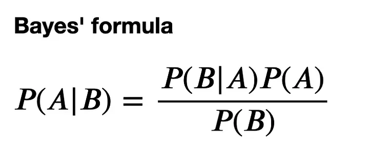
Bayes Theorem
Components:
- P(A|B) — probability of event A given that B occurred
- P(B|A) — probability of event B given that A occurred
- P(A) — prior probability of A (before seeing B)
- P(B) — total probability of B (normalizing constant)
The Three Components in Machine Learning
1 Prior Probability — P(H)
Your initial belief about a hypothesis before observing any data. This encodes existing knowledge, expert opinion, or a uniform assumption if you have none. The prior is your starting point.
2 Likelihood — P(D|H)
The probability of observing the data D given that hypothesis H is true. This is the bridge — it tells you how well each hypothesis explains what you've observed.
3 Posterior Probability — P(H|D)
Your updated belief about hypothesis H after seeing the data D. This is what you actually want — the probability of the hypothesis being true in light of all available evidence.

Example: Disease Diagnosis
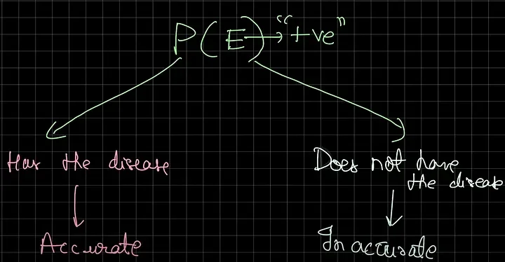
A disease affects 1% of the population. A test for it is 99% accurate. You test positive. What's the probability you actually have the disease?
Intuition says ~99%. Bayes theorem says something quite different.
- Prior: P(disease) = 0.01
- P(positive | disease) = 0.99
- P(positive | no disease) = 0.01
Applying Bayes: P(disease | positive) ≈ 50%. The low base rate (1%) means even a highly accurate test produces many false positives on a healthy population. This is why medical tests often require confirmation.
Example: Horse Race — Hypothesis Convergence
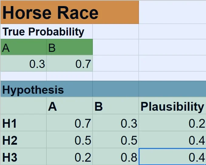
Two horses have actual winning probabilities: Horse A = 0.3, Horse B = 0.7. We start with three hypotheses about their true probabilities. After each race, we update each hypothesis using Bayes theorem.
The hypothesis closest to the true probabilities (A: 0.3, B: 0.7) accumulates the highest posterior after multiple races. False hypotheses gradually lose probability mass.


Why Bayesian Learning Matters
- Incorporates prior knowledge — expert opinions and domain knowledge become priors, not discarded information.
- Quantifies uncertainty — instead of a point prediction, you get a probability distribution, the same instinct behind confidence and prediction intervals in regression.
- Updates dynamically — every new observation refines the posterior without retraining from scratch.
- Principled handling of small data — priors regularize when data is scarce.

Frequently Asked Questions
What is Bayes theorem?
P(A|B) = P(B|A) × P(A) / P(B). It gives you the probability of hypothesis A given evidence B, combining your prior belief P(A) with how likely the evidence is under that hypothesis P(B|A), normalized by total probability of evidence P(B).
What is the difference between prior and posterior probability?
Prior P(H): your belief about hypothesis H before seeing any data. Posterior P(H|D): your updated belief after incorporating observed data D. Bayesian learning is the process of converting priors into posteriors with evidence.
What is likelihood in Bayesian learning?
Likelihood P(D|H) is the probability of observing the data D given hypothesis H is true. It measures how well a hypothesis explains the observed evidence — the bridge between prior and posterior.
Why is Bayesian learning useful in ML?
Bayesian learning incorporates prior knowledge, quantifies uncertainty (outputs distributions, not point predictions), updates dynamically with new data, and handles small datasets via priors as regularization. Used in medicine, spam filtering, fraud detection, NLP, and more.