Confusion Matrix & Metrics Explained
TP, TN, FP, FN, accuracy, precision, recall, F1, specificity — every classification metric defined and applied.
What Is a Confusion Matrix?
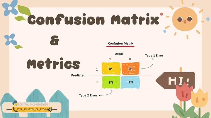
A confusion matrix is a table that describes the performance of a classification model by comparing actual labels with predicted labels. It doesn't reduce performance to one number — it splits every prediction into four categories: true positives (correct positive calls), true negatives (correct negative calls), false positives (false alarms, Type I error), and false negatives (missed detections, Type II error). Every standard classification metric — accuracy, precision, recall, specificity, F1 — is computed directly from these four counts. The matrix matters most on imbalanced data: a model that always predicts "negative" on a 99% negative dataset scores 99% accuracy while catching zero positives, and only the confusion matrix exposes that failure. Read it before trusting any single metric.
The Four Core Elements
TP True Positives
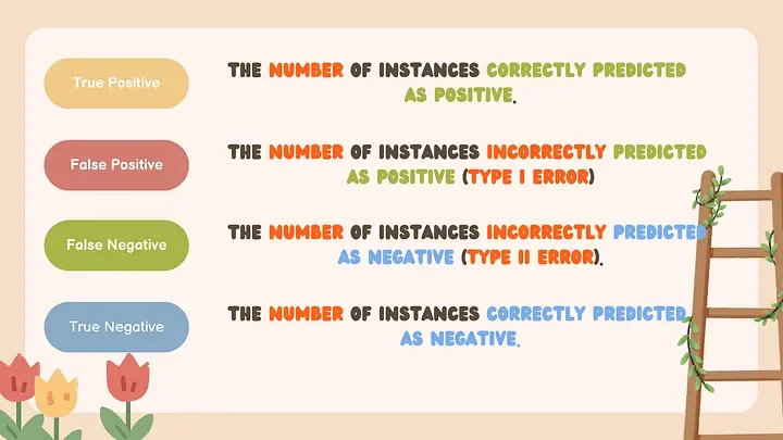
Instances correctly predicted as positive. Model said positive, it was positive. The ideal outcome for positive cases.
TN True Negatives
Instances correctly predicted as negative. Model said negative, it was negative. The ideal outcome for negative cases.
FP False Positives — Type I Error
Instances incorrectly predicted as positive. Model said positive, it was actually negative. "False alarm."
FN False Negatives — Type II Error
Instances incorrectly predicted as negative. Model said negative, it was actually positive. "Missed detection."
The Metrics
1 Accuracy
Overall fraction of correct predictions. Suitable when classes are balanced. On imbalanced datasets, a model predicting "always negative" on a 99% negative dataset achieves 99% accuracy — and catches zero positives. Accuracy is misleading here.

2 Precision
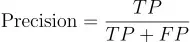
Of all instances the model predicted positive, what fraction actually were? Use when false positives are costly. Example: spam detection — flagging a legitimate email as spam is a false positive with real cost. A drug prescription model — giving a patient a drug they don't need is harmful.

3 Recall (Sensitivity)
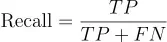
Of all actual positives, what fraction did the model catch? Crucial when false negatives are costly. Example: cancer screening — missing a real case (FN) is far worse than a false alarm. You want to catch every positive, even at the cost of some false positives.

4 F1 Score
The harmonic mean of precision and recall. Balances both when both types of error matter. Preferred over accuracy on imbalanced datasets. A high F1 means both precision and recall are high — the model neither floods with false alarms nor misses real cases.

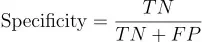
5 Specificity
Of all actual negatives, what fraction were correctly identified as negative? Important in medical diagnostics where correctly classifying healthy patients (true negatives) is critical — avoiding unnecessary treatments.

Worked Example: Pregnancy Diagnosis
Consider a model diagnosing pregnancy (positive = pregnant, negative = not pregnant).

Applied: Breast Cancer Classification Model
A Support Vector Classifier (SVC) trained on the breast cancer dataset demonstrates these metrics in a real scenario. With features from tumor biopsies, the model predicts malignant vs benign.


The full Jupyter notebook with code is available on GitHub Gist:
View Notebook (GitHub Gist)When to Use Which Metric
| Metric | Formula | Answers | Use when |
|---|---|---|---|
| Accuracy | (TP + TN) / total | What fraction of all predictions were correct? | Classes are balanced |
| Precision | TP / (TP + FP) | Of predicted positives, how many were real? | False positives are costly (spam filters, drug prescriptions) |
| Recall (sensitivity) | TP / (TP + FN) | Of actual positives, how many were caught? | False negatives are costly (cancer screening, fraud) |
| Specificity | TN / (TN + FP) | Of actual negatives, how many were correctly cleared? | Avoiding false alarms on healthy/negative cases matters |
| F1 score | 2·(P·R) / (P + R) | Are precision and recall both high? | Imbalanced classes, or both error types matter |
- Balanced classes: accuracy is reliable
- Imbalanced classes: use F1, precision, or recall instead
- FP is costly (spam filter, drug prescription): optimize precision
- FN is costly (cancer screening, fraud detection): optimize recall
- Both errors matter: use F1 as the primary metric
- Medical diagnostics for healthy patients: include specificity
ROC-AUC vs PR-AUC: When Does Each Mislead?
Every metric so far assumes a fixed threshold. Two curve-based metrics evaluate the model across all thresholds at once — and they can tell very different stories on the same model.
The ROC curve plots recall (TPR) against the false positive rate, FPR = FP / (FP + TN), as the threshold sweeps from 1 to 0. ROC-AUC is the area under it — equivalently, the probability that a randomly chosen positive scores higher than a randomly chosen negative. 0.5 is coin-flipping; 1.0 is perfect ranking. The PR curve plots precision against recall over the same sweep, and PR-AUC summarizes that.
Where ROC-AUC misleads: heavy class imbalance. FPR's denominator is all the negatives. With 1% fraud and 99% legitimate transactions, a model can raise thousands of false alarms while FPR barely moves — the mountain of true negatives absorbs them. A fraud model with ROC-AUC 0.95 can still have 10% precision in production: dazzling on the ROC plot, useless to the investigation team. PR-AUC has no TN term anywhere, so it feels every false alarm — on rare-positive problems (fraud, disease screening, defect detection), it is the honest curve.
Where PR-AUC misleads: comparisons across datasets. The PR baseline is the positive prevalence — a random classifier scores PR-AUC ≈ 0.01 at 1% prevalence but ≈ 0.30 at 30%. So a PR-AUC of 0.40 is spectacular in the first setting and mediocre in the second, and comparing PR-AUCs between datasets with different base rates is meaningless. ROC-AUC, being prevalence-invariant, is the fairer cross-dataset yardstick. Rule of thumb: roughly balanced classes → ROC-AUC; rare positives you actively hunt → PR-AUC; ideally report both with the prevalence.
How Do You Choose the Classification Threshold?
Most libraries silently cut at 0.5, but nothing about your problem makes 0.5 special — the threshold is a business decision wearing a statistical costume. Two principled ways to set it:
Youden's J statistic picks the threshold that maximizes J = recall + specificity − 1 — equivalently, the point on the ROC curve farthest above the diagonal. It treats both error types as equally expensive, which makes it a sensible default for screening tests and a common choice in medical diagnostics when no cost information exists.
Cost-based selection admits that errors are rarely symmetric. Assign each error a cost — say a missed fraud case (FN) costs $500 and investigating a false alarm (FP) costs $25 — then, for each candidate threshold, compute the expected cost FP × CFP + FN × CFN from the confusion matrix, and pick the threshold that minimizes it. With a 20:1 cost ratio the optimal threshold drops far below 0.5: you accept many cheap false alarms to avoid expensive misses. The math is trivial; the hard part is getting stakeholders to state the costs out loud — which is itself a useful exercise.
Are Your Predicted Probabilities Calibrated?
Threshold tuning quietly assumes the model's scores mean something: that among cases scored 0.7, about 70% are actually positive. That property is calibration, and many models lack it — modern neural networks are often overconfident, and SVM decision scores aren't probabilities at all. Check it with a reliability diagram (bin predictions by score, plot predicted vs observed positive rate); fix it by post-processing scores with Platt scaling (a logistic fit) or isotonic regression. Calibration matters whenever the probability itself feeds a decision — expected-cost thresholds, risk scores shown to clinicians, bid pricing. It plays the same role for classifiers that confidence and prediction intervals play in regression: honesty about uncertainty, not just a point verdict.
How Do You Average Metrics Across Multiple Classes?
With more than two classes, the confusion matrix becomes N×N, and precision, recall, and F1 are computed per class (one-vs-rest). Reporting a single number then requires choosing how to average — and the choice changes the story:
| Averaging | How it works | What it emphasizes | Use when |
|---|---|---|---|
| Macro | Compute the metric per class, take the unweighted mean | Every class counts equally — rare classes can tank the score | Minority-class performance matters (fraud types, rare diagnoses) |
| Micro | Pool all TP/FP/FN counts globally, then compute once | Every sample counts equally — dominated by frequent classes | Overall throughput matters; equals accuracy in single-label multiclass |
| Weighted | Per-class metric, averaged weighted by class support | A compromise — reflects imbalance but can mask small-class failure | Headline number for imbalanced data, with per-class table alongside |
The gap between macro and micro F1 is itself diagnostic: a model with micro-F1 0.90 but macro-F1 0.55 is excellent on the majority classes and failing the rare ones.
sklearn's classification_report prints all three plus the per-class breakdown — read the per-class rows first, the averages second.
And before averaging anything, confirm the problem really is single-label multiclass rather than multilabel; the setups demand different metrics entirely, as explained in multiclass vs multilabel classification.
Frequently Asked Questions
What is a confusion matrix?
A table comparing actual vs predicted labels across four outcomes: True Positive (TP), True Negative (TN), False Positive (FP — Type I error), False Negative (FN — Type II error). It's the foundation for all classification metrics.
What is the difference between precision and recall?
Precision = TP / (TP + FP) — of predicted positives, how many were real? Use when FP is costly (spam, drug prescription). Recall = TP / (TP + FN) — of all actual positives, how many were caught? Use when FN is costly (cancer, fraud).
What is the F1 score?
F1 = 2 × (Precision × Recall) / (Precision + Recall). Harmonic mean of precision and recall. Preferred over accuracy on imbalanced datasets. A high F1 means the model is both precise and catches most positives.
When should you use accuracy vs F1?
Use accuracy when classes are balanced. Use F1 when imbalanced — a model that always predicts "negative" on a 99% negative dataset achieves 99% accuracy but 0% recall. F1 exposes this failure.
What is specificity?
Specificity = TN / (TN + FP). Of all actual negatives, how many were correctly identified? Critical in medicine for avoiding unnecessary treatment of healthy patients.