Machine LearningSVMKernel Trick

SVMs & Kernel Trick Explained

Support Vector Machines: optimal hyperplane, support vectors, kernel trick, and 4 kernel types with gamma tuning.

July 6, 20255 min readRishabh Singh

Support Vector Machine concept overview — SVM separating data classes — SVMs: find the hyperplane that maximizes the margin between classes.

What Is a Support Vector Machine?

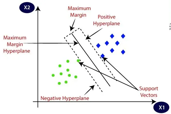
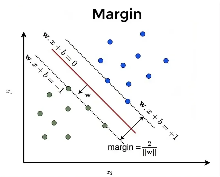
An SVM is a supervised learning algorithm that identifies the optimal hyperplane separating different classes in the feature space. Unlike other classifiers that just find any boundary that works, an SVM finds the one with the maximum margin — the widest gap between the boundary and the closest data points on either side.

Those closest points are called support vectors. They're the only data points that actually influence the boundary — everything else is irrelevant to the decision surface.

SVM decision boundary with maximum margin hyperplane and support vectors — The SVM hyperplane (solid line) maximizes the margin (dashed lines). Support vectors are the closest points to the boundary.

The Problem: Non-Linearly Separable Data

A straight hyperplane works fine when classes are cleanly separable. But real data is rarely that cooperative. When classes form rings, spirals, or overlapping clusters, no straight line can separate them.

Non-linearly separable data — two classes that cannot be separated by a straight line — Non-linearly separable data: no straight hyperplane can cleanly divide these classes.

The Solution: The Kernel Trick

Instead of drawing a curved boundary in low-dimensional space, the kernel trick projects the data into a higher-dimensional feature space where a straight hyperplane can separate the classes.

The key insight: you never actually compute the coordinates in that high-dimensional space. Kernels compute the dot products in the transformed space directly from the original inputs — giving you the power of high-dimensional separation at low computational cost.

"The kernel trick lets SVMs separate non-linear data without ever explicitly computing the transformation."

Kernel trick: data projected from 2D to 3D space where it becomes linearly separable — Kernel trick: project into higher dimensions → straight hyperplane becomes possible.

The 4 Kernel Types

1 Linear Kernel

No transformation — computes a standard dot product in the original feature space. Use when data is already linearly separable. Fast, interpretable, no hyperparameters to tune.

K(x, y) = x · y

Linear SVM kernel — straight hyperplane separating two classes — Linear kernel: works only when classes are linearly separable.

2 Polynomial Kernel

Maps data into a polynomial feature space. With degree 2, it considers not just original features but also their squares and cross-products (x², y², xy). Captures feature interactions that a linear kernel misses.

K(x, y) = (x · y + c)ᵈ

Polynomial SVM kernel — curved decision boundary capturing feature interactions — Polynomial kernel: curved boundaries from feature interactions — degree controls complexity.

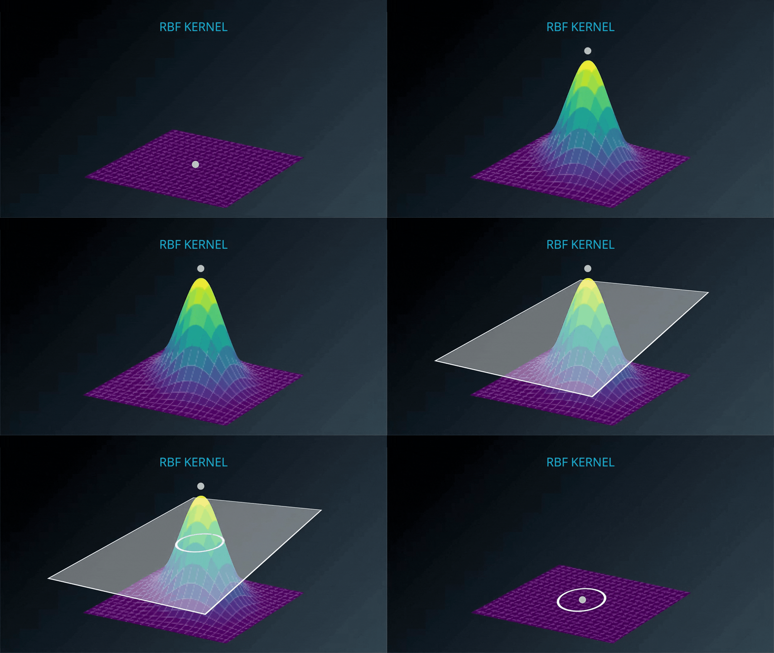
3 RBF — Radial Basis Function Kernel

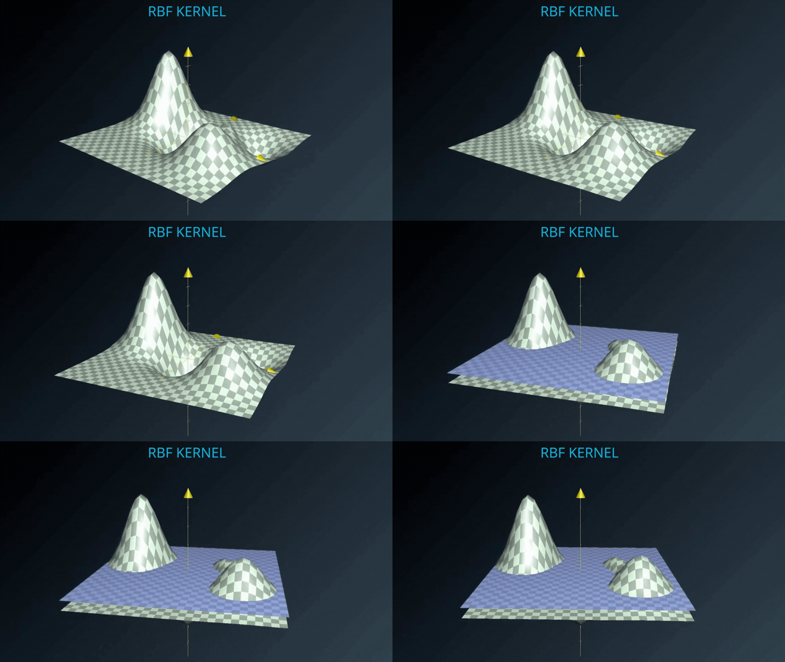
The default kernel in sklearn's SVM. Computes similarity between points using Euclidean distance — points closer together get higher similarity scores. Maps data into infinite-dimensional space, making it extremely flexible for complex boundaries.

K(x, y) = exp(−γ ‖x − y‖²)

RBF kernel animation — SVM decision boundary adapting to complex data shapes — RBF kernel animation: the boundary wraps tightly around complex data distributions.

Tuning Gamma (γ) in RBF

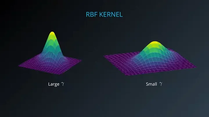
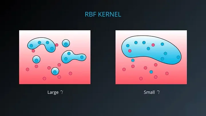
Gamma controls the influence radius of each training point — how far a single example reaches.

High γ

Each point influences only its immediate neighborhood. The boundary hugs the training data tightly, capturing fine-grained detail. Risk: overfitting.

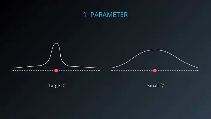
High gamma SVM — overly complex decision boundary that hugs training points — High γ: boundary memorizes the training data — good fit, poor generalization.

Low γ

Each point influences a wide area. The boundary is smooth and generalized. Risk: underfitting when data has complex structure.

Low gamma SVM — overly smooth decision boundary that misses local structure — Low γ: boundary is too smooth — misses local structure, may underfit.

4 Sigmoid Kernel

Uses the hyperbolic tangent function — similar to the activation function in neural networks. Produces S-shaped decision boundaries. Less commonly used than RBF but useful when the data exhibits neural-network-like behavior.

K(x, y) = tanh(αx · y + c)

Sigmoid kernel SVM animation — S-shaped decision boundary — Sigmoid kernel: mimics neural network activation, produces non-linear S-shaped boundaries.

Kernel Comparison at a Glance

Summary comparison of Linear, Polynomial, RBF, and Sigmoid SVM kernels — Kernel summary: choose based on data linearity, complexity, and the need for interpretability.

Key Takeaways

SVM goal: find the hyperplane that maximizes the margin between classes — not just any separating boundary.
Support vectors are the only training points that matter — the rest can be removed without changing the boundary.
Kernel trick: maps data to higher dimensions implicitly, enabling linear separation of non-linear data at low compute cost.
RBF is the default in sklearn — flexible for most problems; tune γ and C via cross-validation.
High γ → overfitting. Low γ → underfitting. GridSearchCV over γ and C is the standard approach.

For the applied side — training an SVC on the Iris dataset and tuning C, gamma, and kernels with real scores — see Support Vector Machine (SVM).

Frequently Asked Questions

What is a Support Vector Machine?

An SVM finds the optimal hyperplane that separates different classes in the feature space, maximizing the margin between the closest data points (support vectors) of each class.

What is the kernel trick in SVM?

The kernel trick maps non-linearly separable data into a higher-dimensional feature space where it becomes linearly separable — without ever explicitly computing the coordinates in that high-dimensional space. This makes SVMs efficient even with complex, curved decision boundaries.

What are the different SVM kernels?

The four main kernels: (1) Linear — standard dot product, for linearly separable data; (2) Polynomial — captures squares and cross-products of features; (3) RBF — default in sklearn, Euclidean distance similarity; (4) Sigmoid — mimics neural network activation.

What does gamma do in RBF SVM?

Gamma controls influence radius per training point. High γ: tight, complex boundaries that capture fine detail — risks overfitting. Low γ: smooth, simple boundaries — risks underfitting.

When should you use SVM over other classifiers?

SVMs excel in high-dimensional spaces, when features outnumber samples, and when a clear margin exists. Strong for text classification, image recognition, bioinformatics. They scale poorly on very large datasets — consider gradient-boosted trees or neural networks then.

Back to Blog Read on Medium