Machine LearningPython

Support Vector Machine (SVM)

SVM: hyperplanes, margins, support vectors, C and gamma tuning, 4 kernels, and Iris dataset implementation with scikit-learn.

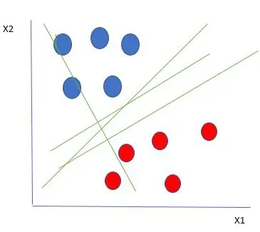
September 15, 20235 min readRishabh Singh

Support Vector Machine — decision boundary with maximum margin — SVM: a powerful algorithm for linear and non-linear classification, regression, and outlier detection.

What is a Support Vector Machine?

A Support Vector Machine (SVM) is a supervised machine learning algorithm used for linear or non-linear classification, regression, and outlier detection. The core idea: find the hyperplane that best separates two classes with the maximum possible margin between them.

Hyperplane and Margins

In 2D, a hyperplane is a line. In 3D, it's a plane. In N dimensions, it's an (N−1)-dimensional boundary that separates classes. SVM doesn't just find any separating line — it finds the one that maximizes the margin to the nearest data points on each side.

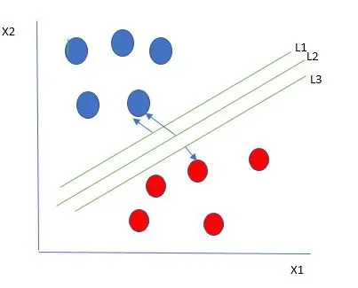
SVM hyperplane with margins L1, L2, L3 — Three candidate boundaries: L1 and L3 are soft margins; L2 is the hard margin (optimal hyperplane).

L1, L3 — Soft margins: closer to data points, smaller margin
L2 — Hard Margin / Hyperplane: maximum margin, optimal choice when data is linearly separable

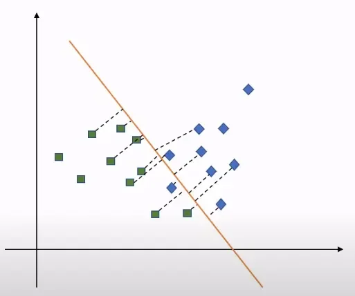
SVM maximum margin hyperplane visualization — The optimal hyperplane maximizes the distance to the nearest data point on each side.

Support Vectors

Support vectors are the data points closest to the margin boundary. They are the critical points that define the margin — if you removed them, the hyperplane would shift. The algorithm name comes from these vectors: the machine is "supported" by these boundary points.

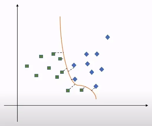
Hard margin vs soft margin SVM comparison — Hard margin (no violations) vs soft margin (some misclassifications allowed for better generalization).

Regularization (C) and Gamma

Two key hyperparameters tune SVM performance. High values in complex datasets can cause overfitting.

Regularization (C)

The C parameter controls the trade-off between maximizing the margin and minimizing misclassification. A larger C penalizes misclassifications more heavily — narrower margin, more accurate on training data, higher risk of overfitting. A smaller C tolerates more misclassifications — wider margin, better generalization.

Effect of C parameter on SVM margin width — Higher C → narrower margin with fewer misclassifications. Lower C → wider margin, more tolerant.

Gamma

Gamma controls the influence radius of individual training points in non-linear kernels (RBF, Polynomial, Sigmoid). High gamma: each point influences only a small region — complex, tight boundaries (overfitting risk). Low gamma: each point influences a large region — smoother, simpler boundaries.

SVM C and gamma interaction visualization — C and gamma interact: tuning both together determines the complexity and generalization of the SVM boundary.

Kernels

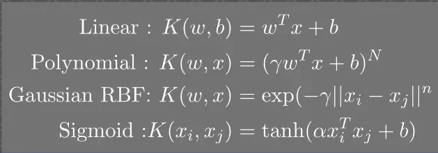
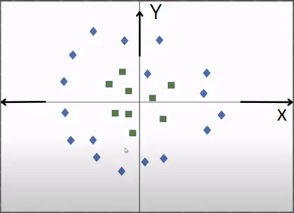
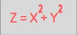
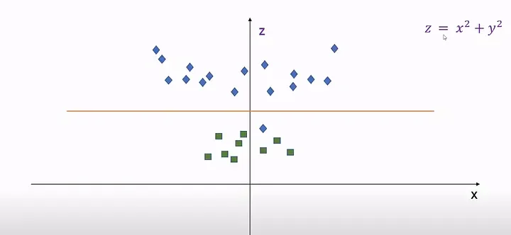
Most real-world data isn't linearly separable. Kernels are mathematical functions that implicitly transform data into a higher-dimensional space where a linear hyperplane can separate it — without explicitly computing the transformation.

Non-linearly separable data transformed by kernel — Kernels map data to higher dimensions where a linear boundary becomes possible.

Four Kernels

Linear: K(x, y) = x·y — for linearly separable data, fastest, no transformation
Polynomial: K(x, y) = (γx·y + r)^d — captures feature interactions up to degree d
RBF (Radial Basis Function): K(x, y) = exp(−γ||x−y||²) — the default, works well for most problems, infinite-dimensional mapping
Sigmoid: K(x, y) = tanh(γx·y + r) — similar to neural network activation, less common

Linear kernel SVM decision boundary — Linear kernel: optimal for linearly separable data — fastest computation, highest interpretability.

RBF kernel SVM — non-linear decision boundary — RBF kernel: creates non-linear boundaries by computing Gaussian distance to each support vector.

Polynomial and Sigmoid kernel SVM boundaries — Polynomial kernel captures interactions between features; Sigmoid mirrors neural network behavior.

Implementation: Iris Dataset

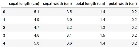
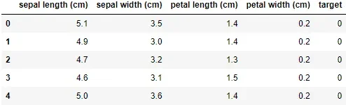
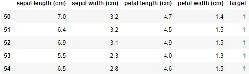
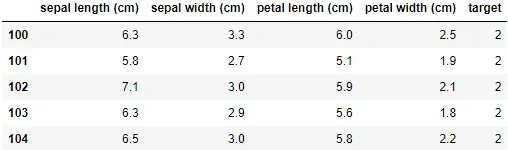
Load the Iris dataset and train an SVM classifier. Three species make this a multiclass problem — sklearn's SVC handles it with a one-vs-one strategy under the hood:

import pandas as pd
from sklearn.datasets import load_iris

iris = load_iris()
# Features: sepal length, sepal width, petal length, petal width
# Classes: setosa, versicolor, virginica

df = pd.DataFrame(iris.data, columns=iris.feature_names)
df['target'] = iris.target
df['flower_name'] = df.target.apply(lambda x: iris.target_names[x])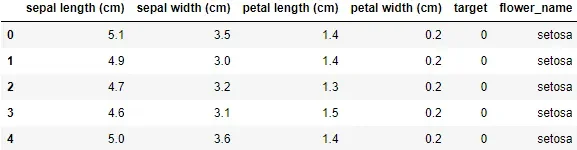

Iris dataset scatter plot — petal length vs petal width — Iris dataset: petal features show clear separation between setosa and the other two classes.

from sklearn.model_selection import train_test_split
from sklearn.svm import SVC

X = df.drop(['target', 'flower_name'], axis='columns')
y = df.target
X_train, X_test, y_train, y_test = train_test_split(X, y, test_size=0.2)

model = SVC()
model.fit(X_train, y_train)
model.score(X_test, y_test)
# 0.9666666666666667

model.predict([[4.8, 3.0, 1.5, 0.3]])
# array([0])  → setosa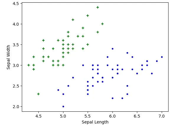

SVM model training on Iris dataset output — Default SVC achieves ~96.7% accuracy on the Iris test set.

Tuning Hyperparameters

# Regularization (C)
model_C = SVC(C=1)
model_C.fit(X_train, y_train)
model_C.score(X_test, y_test)   # 0.9666

model_C = SVC(C=10)
model_C.fit(X_train, y_train)
model_C.score(X_test, y_test)   # 0.9666

# Gamma
model_g = SVC(gamma=10)
model_g.fit(X_train, y_train)
model_g.score(X_test, y_test)   # 0.9333 — overfitting with high gamma

# Kernels
model_linear = SVC(kernel='linear')
model_linear.fit(X_train, y_train)
model_linear.score(X_test, y_test)   # 1.0 — perfect on Iris

model_rbf = SVC(kernel='rbf')   # default
model_rbf.fit(X_train, y_train)
model_rbf.score(X_test, y_test)  # 0.9666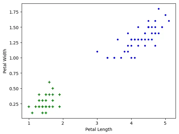

SVM hyperparameter tuning results — C, gamma, kernel comparison — Linear kernel achieves 100% on Iris — the dataset is linearly separable in 4D feature space.

"The linear kernel achieves 100% accuracy on Iris because the 4-dimensional feature space is linearly separable — the kernel trick maps apparent non-linearity in 2D to separability in higher dimensions."

One caution before shipping a score like 96.7%: accuracy alone can hide class-level failures. Inspect the full confusion matrix and per-class precision and recall before trusting any single number.

See also: SVMs & Kernel Trick in a Minute — a deeper dive into the mathematics behind SVM kernels.

Back to Blog Read on Medium