Linear Regression Explained
y=mx+b, cost function (MSE), gradient descent, R² score, multivariable regression — with Python implementation.

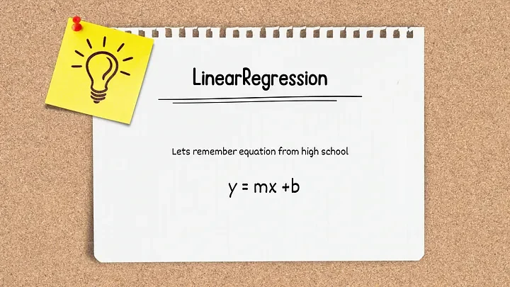
The Foundation: y = mx + b
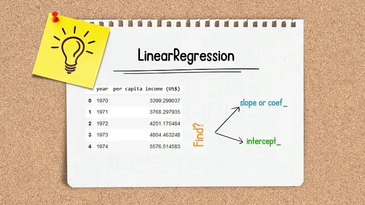
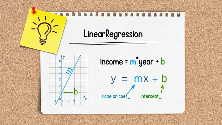
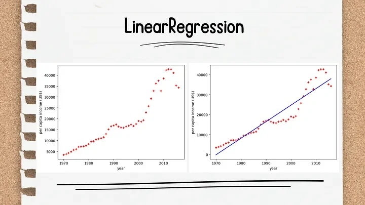
Linear regression starts from the same equation you learned in school. Given data points (years, income), the goal is to find the line that best fits them — the one that minimizes prediction error across all points. This is the workhorse behind causal forecasting — predicting an outcome from its drivers.
θ₀ is the intercept (y-axis offset), θ₁ is the slope. The model learns these parameters from data.
The Cost Function
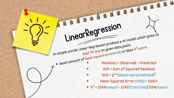
How do you measure how "wrong" the line is? The cost function quantifies total prediction error across all training examples. Linear regression uses Mean Squared Error (MSE) — also called Least Squared Error.
Squaring errors serves two purposes: negative errors don't cancel positive ones, and large errors are penalized more severely than small ones.
Gradient Descent
Gradient descent finds the parameters θ that minimize J(θ). Starting from a random point, it computes the gradient (slope of the cost function surface) and takes a step downhill. Repeat until convergence.
α is the learning rate — too large and it overshoots, too small and it converges slowly.

Evaluation Metrics
Mean Absolute Error (MAE)
Average absolute difference. Interpretable in original units. Less sensitive to outliers than MSE.
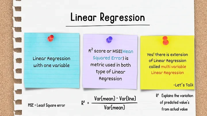
R² Score (Coefficient of Determination)
Explains the proportion of variance in the target explained by the model. R² = 1 means perfect fit; R² = 0 means the model does no better than predicting the mean.
Multivariable Linear Regression
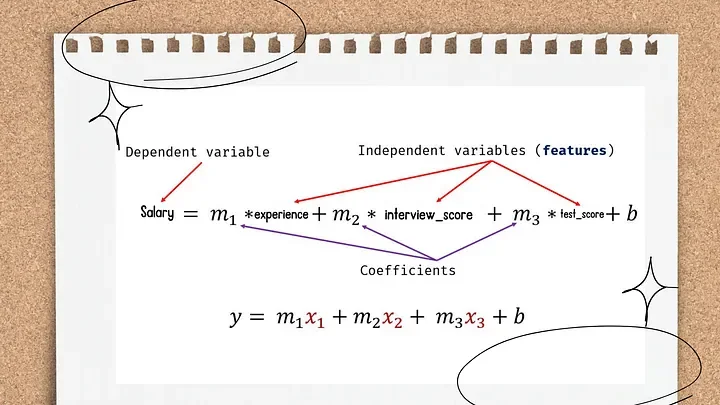
Real datasets have multiple features. Multivariable linear regression extends the hypothesis to many input dimensions:
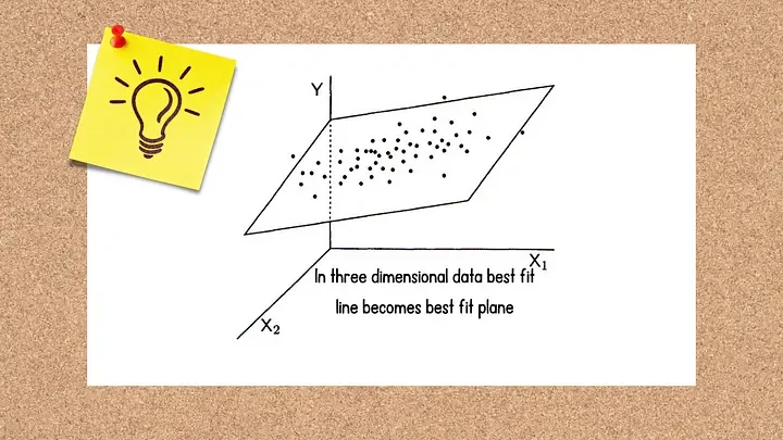
With 2 features, the model fits a plane instead of a line. With 3+ features, it fits a hyperplane — no longer visualizable, but the math is identical (the same hyperplane concept that SVMs use as a decision boundary). Whatever the dimension, the model outputs point estimates — to quantify how uncertain they are, wrap them in confidence and prediction intervals.
Implementation Notebooks
Full implementations available on GitHub Gist:
Key Takeaways
- Hypothesis: ŷ = θ₀ + θ₁x — a line (or hyperplane) parameterized by θ.
- Cost function (MSE): measures total squared error — what gradient descent minimizes.
- Gradient descent: iteratively adjusts θ downhill on the cost surface.
- R² score: how much variance the model explains — closer to 1 is better.
- Multivariable: same algorithm, extra θs — fits a plane or hyperplane instead of a line.